Oman_NGS
Bacterial genome assembly using Mycobacterium tuberculosis example dataset
Table of contents
1. Introduction
In this module, we are going to work through how to generate SARS-CoV-2 consensus genomes from Oxford Nanopore data. The most popular pipeline for this is called ARTIC.
You can find more information here:
ARTIC : https://github.com/artic-network/fieldbioinformatics
We will
- Use
gitto pull data from a github account - Compare assembly methods using
quast - Use
prokkato annotate genomes - Learn the assembly commands for SKESA and Spades
First we need to download the assembly datasets that I have run
cd Oman_modules
git pull
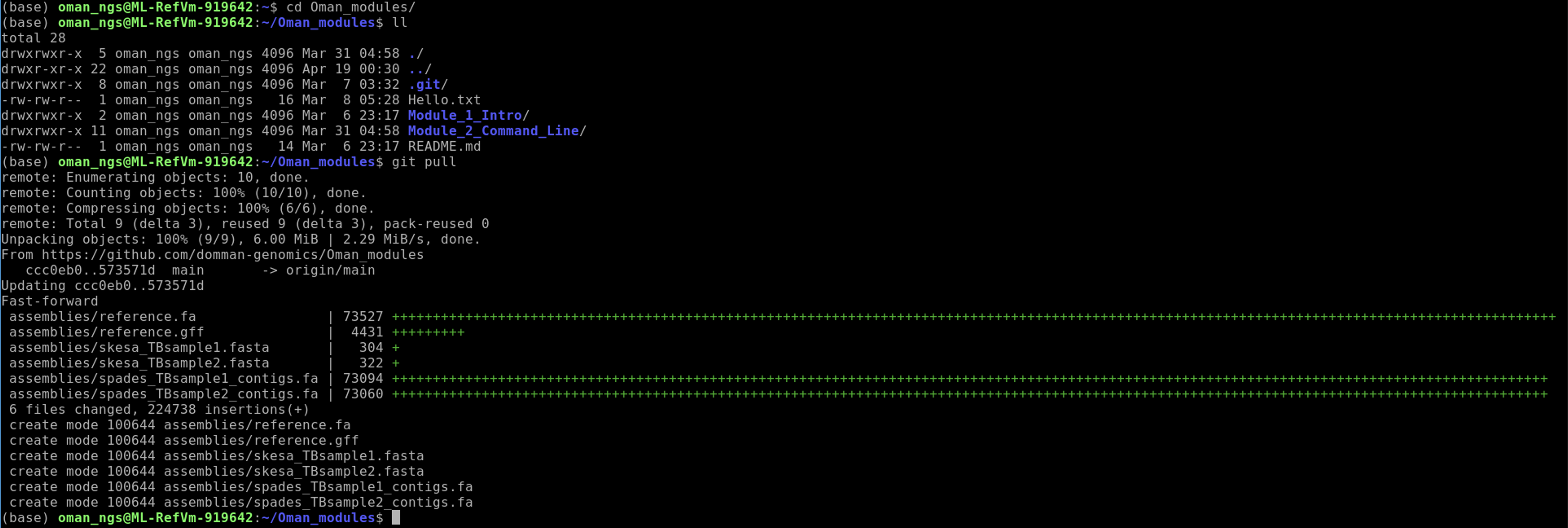
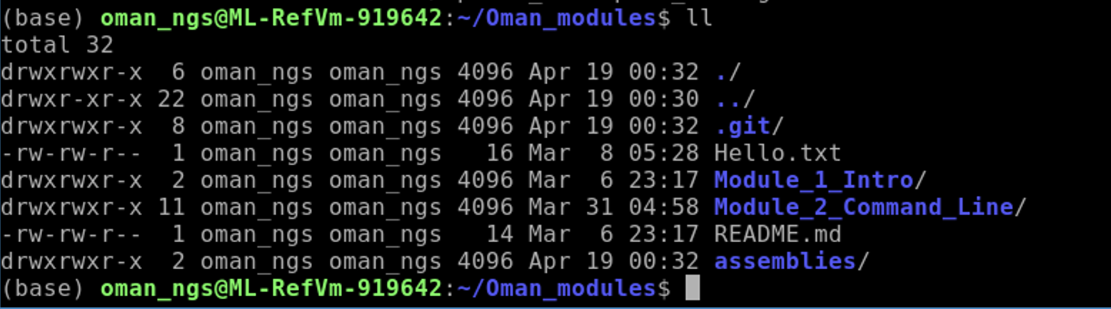
Check to see we now have an assembly folder:
ll
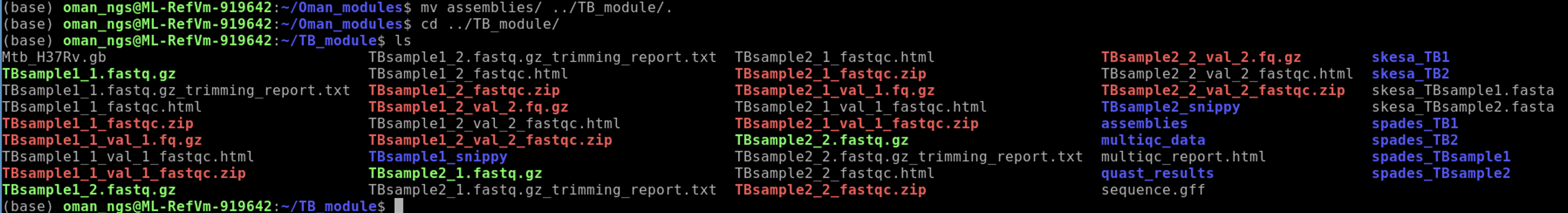
Now move the assemblies folder to our TB_module folder:
mv assemblies/ ../TB_module/.
cd ../TB_module
ls
You should see the assemblies folder in now in the TB_module folder.
We are now ready to use quast to compare the assemblies
Compare assemblies using Quast
First move into the TB dataset assemblies folder we just downloaded:
cd assemblies
We need to install Quast by creating a new conda environments
We will be using a program called Quast to assess the quality of assemblies : https://github.com/ablab/quast
Install mamba by using the following command:
mamba create -n quast -y -c conda-forge -c bioconda quast
mamba create : command that creates a new environment
-n quast : create new environment called quast
-c conda-forge: adds conda-forge channel
-c bioconda: adds bioconda channel
quast : installs quast package
Once it has finished installing you can now activate the environment by typing:
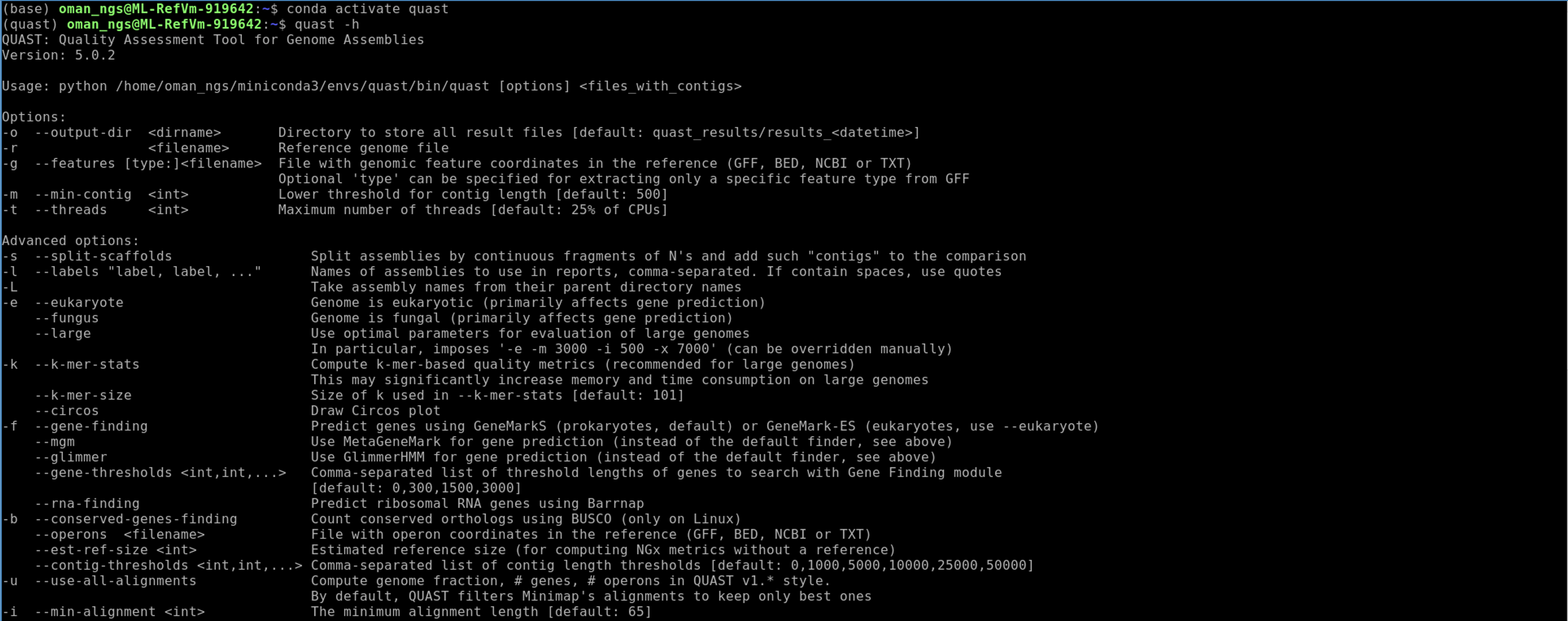
conda activate quast
Check quast is installed properly and get an idea of how to run the program:
quast -h
This should do the trick, and everything should work now.
Run quast on our assemblies:
Quast usage is as follows:
quast [options] <contig files>
Contig files are the .fasta or .fa files produced by assembly programs
quast -l skesa_TB1,skesa_TB2,spades_TB1,spades_TB2 skesa_TBsample1.fasta skesa_TBsample2.fasta spades_TBsample1_contigs.fa spades_TBsample2_contigs.fa
-l : you can rename what the assembly dataset is called here. We do this to make it easier when we are looking at the results instead of long names
Use firefox to look at the output files:
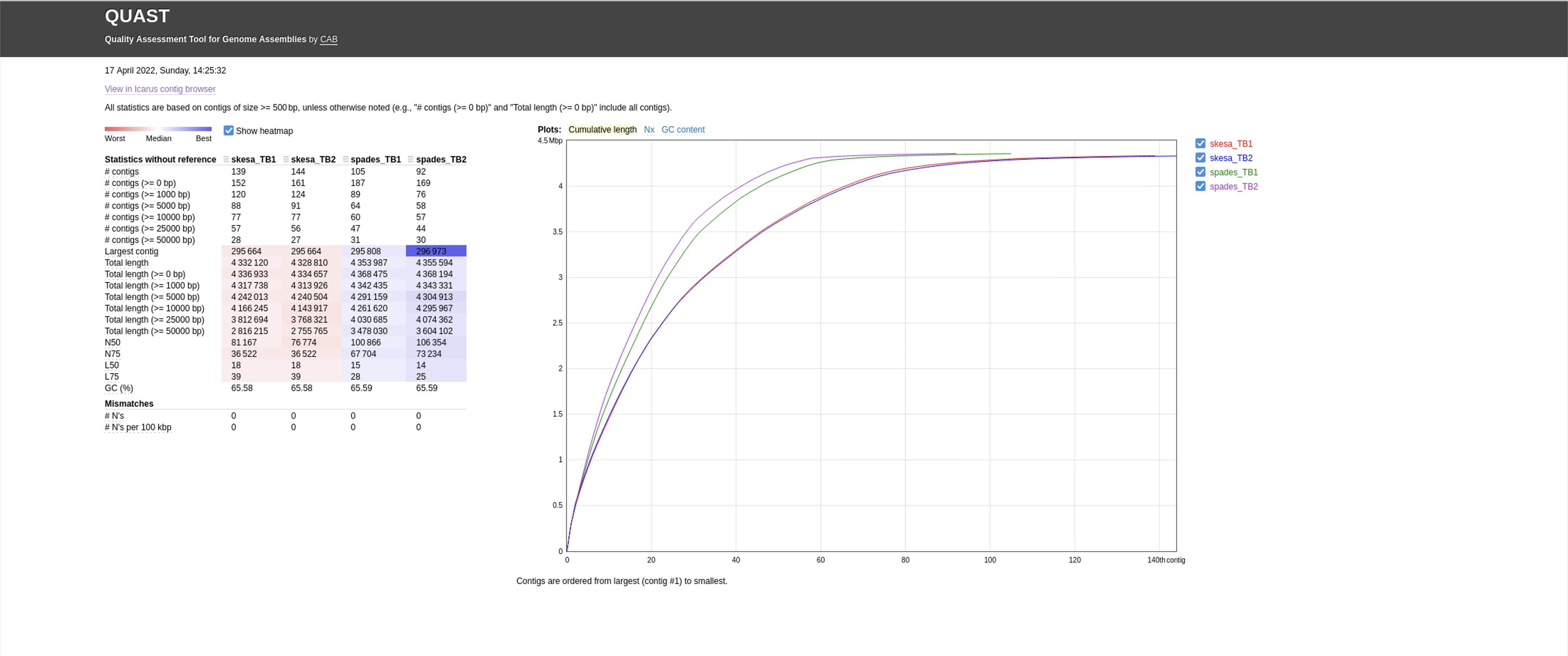
firefox quast_results/latest/report.html
There are a number of useful metrics reported by Quast on each assembly:
- Total number of contigs
- Largest contig
- Total length of the assembly
- N50 value : the length of the shortest contig for which longer and equal length contigs cover at least 50 % of the assembly
Compare the SKESA versus Spades assemblies for TB1 and TB2 datasets.
Questions
- For each dataset (TB1 and TB2), which assembler produces more contigs?
- For each dataset (TB1 and TB2), what is the size difference between the assemblies?
- Do you notice a trend between the assemblers?
You can also run quast using a reference genome which can give more insight into the differences between the assemblies:
quast -r reference.fa -g reference.gff -l skesa_TB1,skesa_TB2,spades_TB1,spades_TB2 skesa_TBsample1.fasta skesa_TBsample2.fasta spades_TBsample1_contigs.fa spades_TBsample2_contigs.fa

firefox quast_results/latest/report.html
2. Run prokka to annotate genomes
Prokka is a very popular (probably the most) bacterial annotation tool. You can read more about it here : https://github.com/tseemann/prokka
First we need to create a new environment and install prokka:
mamba create -n annotate -c conda-forge -c bioconda -c defaults prokka
conda activate annotate
Now run prokka
prokka --cpus 4 --proteins ../Mtb_H37Rv.gb --outdir skesa_TB1 --prefix TB1_skesa skesa_TBsample1.fasta
prokka --cpus 4 --proteins ../Mtb_H37Rv.gb --outdir skesa_TB2 --prefix TB2_skesa skesa_TBsample2.fasta
There are many output files produced by prokka:
Output Files
| Extension | Description |
|---|---|
| .gff | This is the master annotation in GFF3 format, containing both sequences and annotations. It can be viewed directly in Artemis or IGV. |
| .gbk | This is a standard Genbank file derived from the master .gff. If the input to prokka was a multi-FASTA, then this will be a multi-Genbank, with one record for each sequence. |
| .fna | Nucleotide FASTA file of the input contig sequences. |
| .faa | Protein FASTA file of the translated CDS sequences. |
| .ffn | Nucleotide FASTA file of all the prediction transcripts (CDS, rRNA, tRNA, tmRNA, misc_RNA) |
| .sqn | An ASN1 format “Sequin” file for submission to Genbank. It needs to be edited to set the correct taxonomy, authors, related publication etc. |
| .fsa | Nucleotide FASTA file of the input contig sequences, used by “tbl2asn” to create the .sqn file. It is mostly the same as the .fna file, but with extra Sequin tags in the sequence description lines. |
| .tbl | Feature Table file, used by “tbl2asn” to create the .sqn file. |
| .err | Unacceptable annotations - the NCBI discrepancy report. |
| .log | Contains all the output that Prokka produced during its run. This is a record of what settings you used, even if the –quiet option was enabled. |
| .txt | Statistics relating to the annotated features found. |
| .tsv | Tab-separated file of all features: locus_tag,ftype,len_bp,gene,EC_number,COG,product |
The GenBank .gbk file is one of the main outputs that is usefull for downstream applications, as is the .gff file.
3. Viewing assemblies in genome browser
You can take an interactive look at your genomes by using one of several interactive genome browsers. My personal favorite is artemis, but another popular one is IGV.
You can load your annotated genome for viewing in Artemis like so:
conda activate base
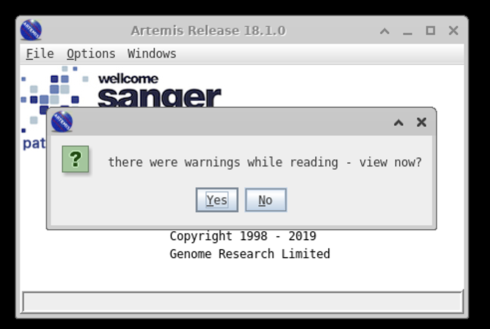
art skesa_TB1/TB1_skesa.gff
When you first start this up an annoying box will appear telling you Artemis is complaining about something and that there are warnings. In this case hit the NO button.
You should now be on the main screen.
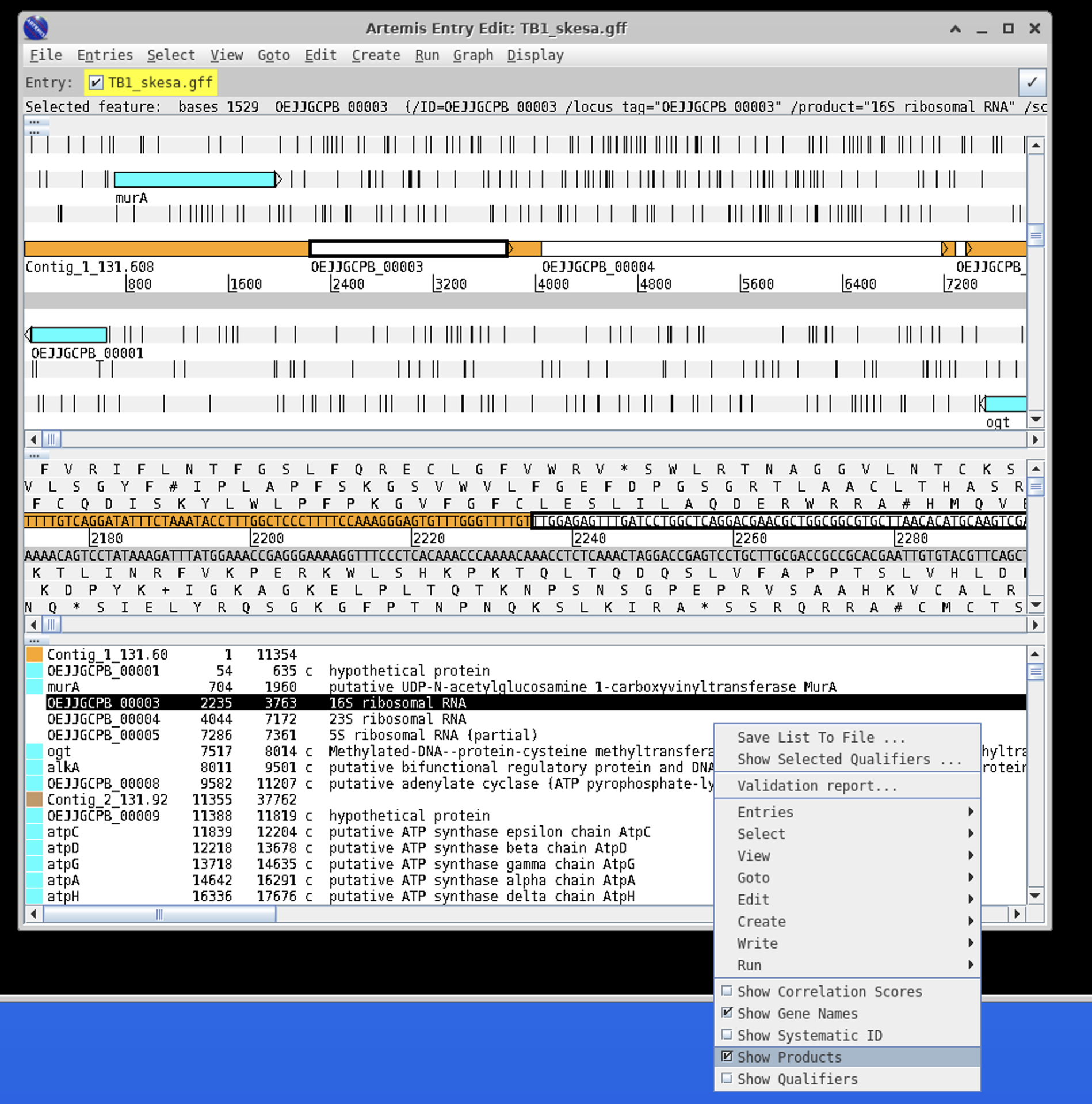
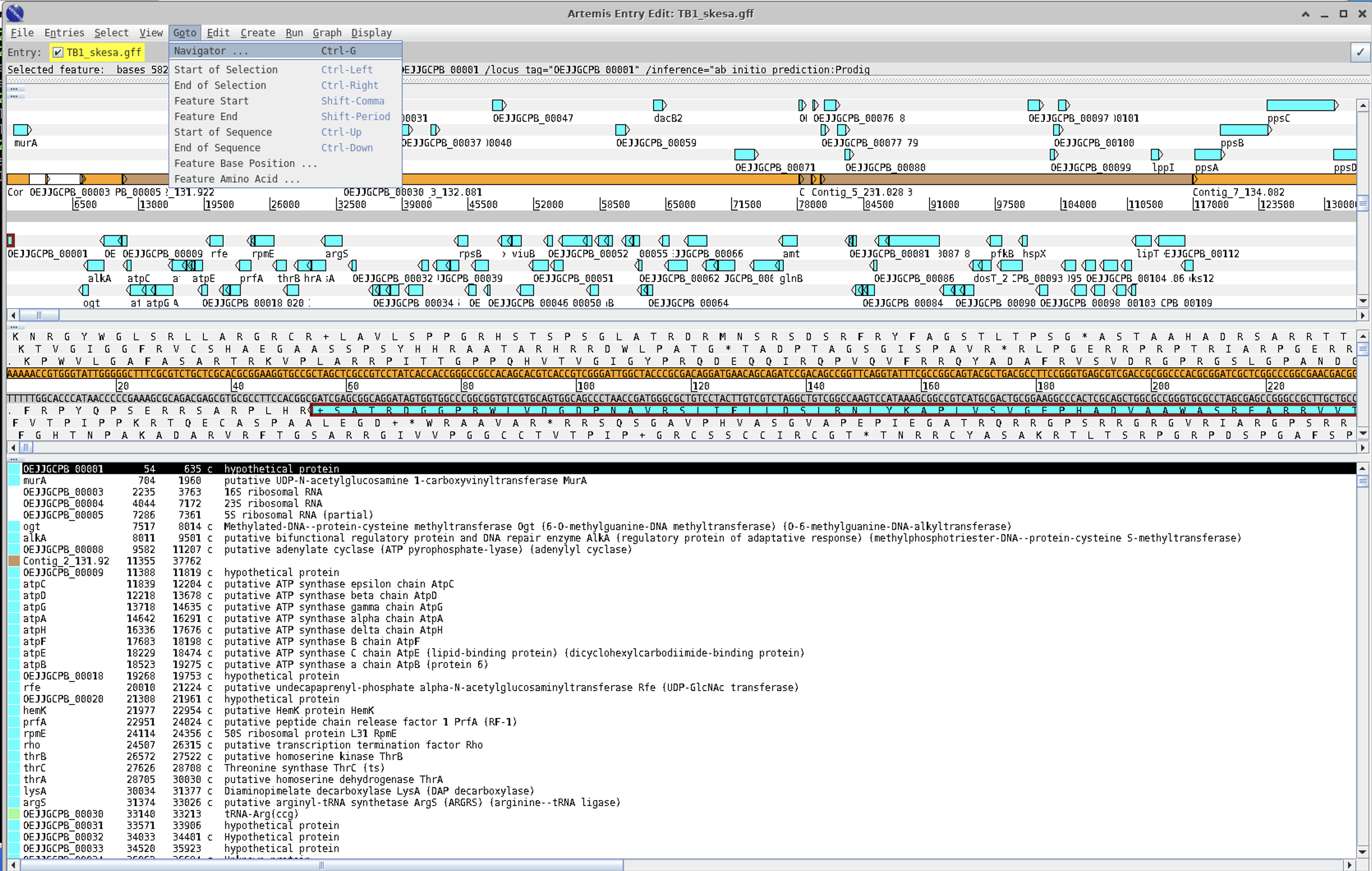
A few things are helpful when browsing. Right click in the white area to the right on the bottom panel to bring up the following menu:
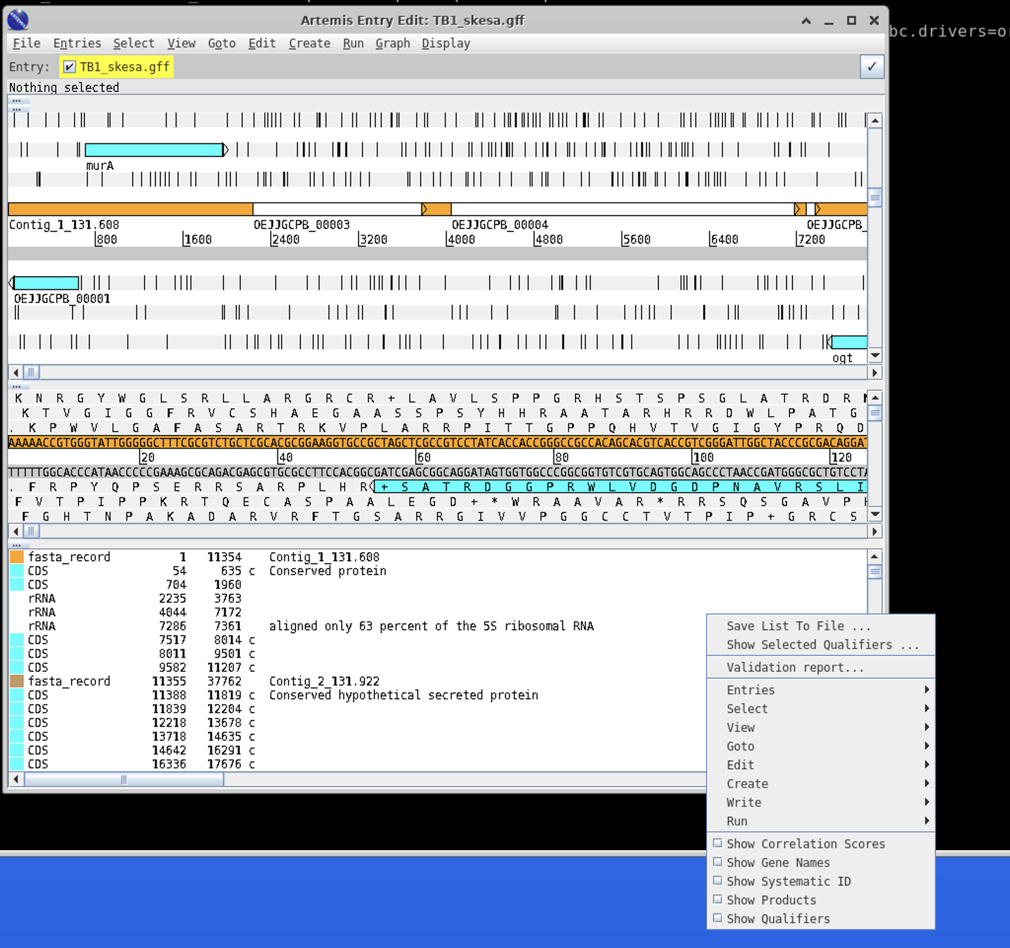
Click Show Gene Names and Show Products
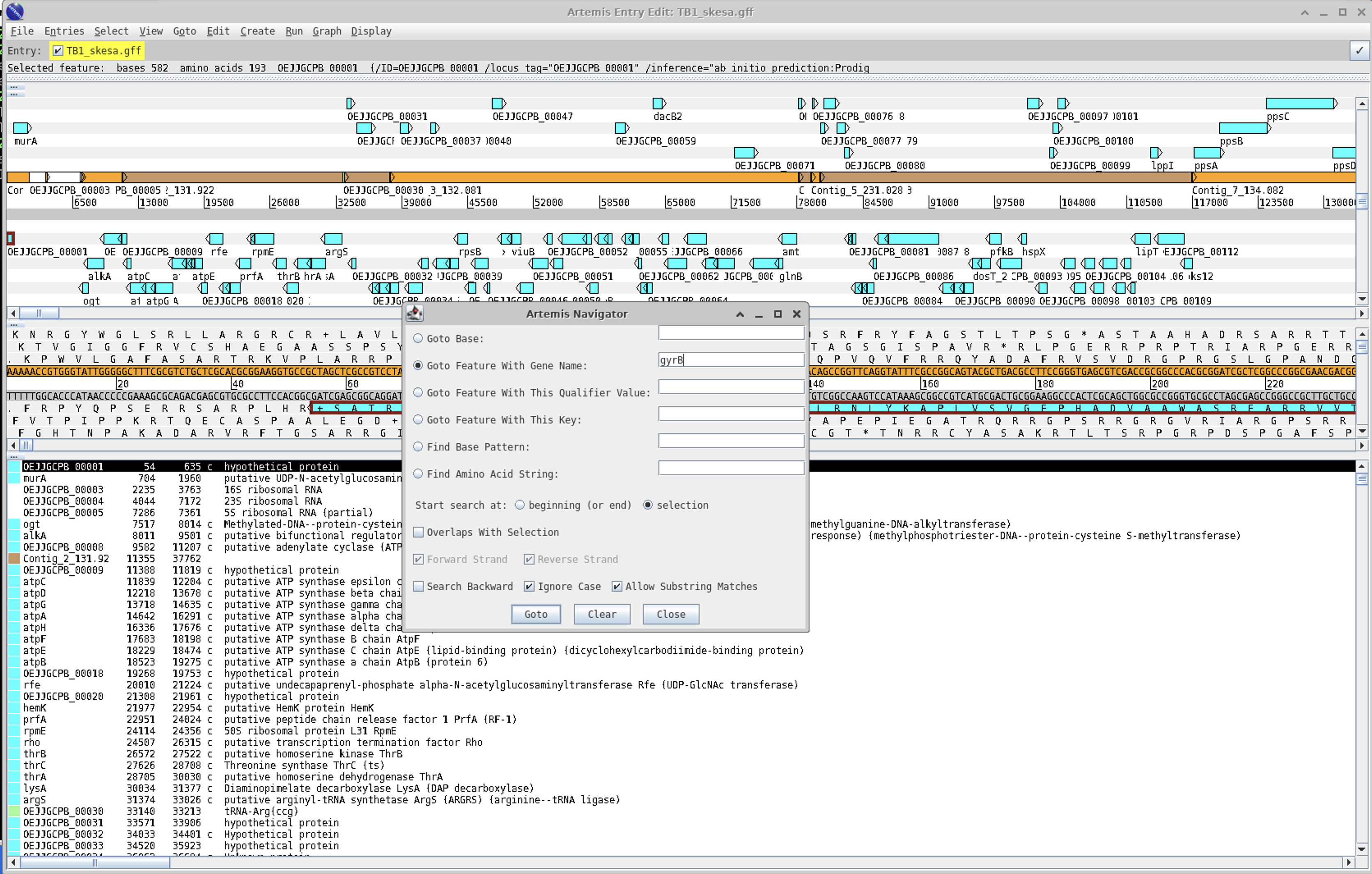
A very useful tool is the navigation pane within Artemis.
For instance, if we wanted to find the gyrB gene you can search for it as follows:
A full in-depth review of Artemis is just not possible within our 90 minutes, but you can look at a module from a course that I have taught on for a numner of years for more background : https://github.com/domman-genomics/WWPG_2022/blob/main/manuals/module_artemis/module_artemis.md
4. Commands for running bacterial genome assembly
You do not need to run these commands! They are here for informational purposes.
Two very popular bacterial genome assembly programs are SKESA and Spdaes. A popular tool for running spades assemblies is called shovill which is what we are using here.
You can find more information here:
SKESA : https://github.com/ncbi/SKESA
Shovill : https://github.com/tseemann/shovill
First we install the programs in a new conda environment:
mamba create -n assembly -c bioconda -c conda-forge skesa shovill
conda activate assembly
Run the skesa assembler : ~20 minutes per dataset
skesa --reads TBsample1_1_val_1.fq.gz,TBsample1_2_val_2.fq.gz --cores 4 --memory 8 > skesa_TBsample1.fasta
skesa --reads TBsample2_1_val_1.fq.gz,TBsample2_2_val_2.fq.gz --cores 4 --memory 8 > skesa_TBsample2.fasta
Run shovill aka spades assembler : ~35 minutes per dataset
shovill --outdir spades_TBsample1 --R1 TBsample1_1_val_1.fq.gz --R2 TBsample1_2_val_2.fq.gz
shovill --outdir spades_TBsample2 --R1 TBsample2_1_val_1.fq.gz --R2 TBsample2_2_val_2.fq.gz